Created: 02 December 2000 Updated:29 May 2011: some minor changes.
This essay is entirely my own thoughts, so the standard disclaimers apply. I'm writing a Web essay rather than a formal publication because I doubt this material is worthy of even a "Note" in some journal. Instead, I'm hoping to correct some possible misuse of the virtual temperature correction. Hopefully, this clears up any misunderstandings. If any remain, you can contact me at cdoswell # earthlink.net [use the email hyperlink or cut out the " # " and replace it with "@"].
In 1994, Erik Rasmussen and I published a short paper on the use of the virtual temperature correction for calculating convective available potential energy [CAPE].
Doswell, C.A. III, and E.N. Rasmussen, 1994: The effect of neglecting the virtual temperature correction on CAPE calculations. Wea. Forecasting, 9, 619-623.
It recently has come to my attention that there may be some continuing confusion about precisely how to apply the virtual correction to the problem of calculating CAPE and other parameters (such as convective inhibition [CIN], the lifting condensation level height [LCL], the level of free convection [LFC] height, or the equilibrium level [EL] height).
Therefore, I want to begin this discussion with some tutorial material, before I go on to the specific issues. An excellent treatment of the topic can be found in Hess (1959; §4.3):
Hess, S.L., 1959: Introduction to Theoretical Meteorology. Holt, Rhinehart, and Winston, 362 pp.
Just what is the virtual correction? What purpose does it serve? The Equation of State should be familiar to most of my readers; it is:
where p is the pressure, r is the density, R is the so-called Gas Constant (see below), and T is the temperature. I'm not going to go into the issue of units here, although they can be tricky, because most meteorologists think of pressure in terms of millibars, which makes things a little difficult. The issue in applying this version of the Equation of State is that the Gas Constant is not exactly constant, when the gas involves a mixture of air (which is, in turn, a mixture comprising mostly nitrogen, oxygen, argon, and carbon dioxide) with some highly variable amount of water vapor.
In the troposphere, the relative percentages of the dry components in air remain pretty much constant (ignoring the anthropogenic increase in CO2) and so dry air has, in fact, a pretty much constant value for its Gas Constant, Rd, where the subscript denotes the fact that it applies only to dry air. Each gaseous constituent has a different Gas Constant, but since the mixture remains the same, a single value of the Gas Constant can be found for the mixture. Adding water vapor to the mixture wouldn't be a problem if the percentage of water vapor within the mixture remained fixed; but it clearly changes over a wide range of mixing ratios.
The mixing ratio, q, is defined as the mass of water vapor per unit mass of dry air:
where p is the total air pressure, e is the partial pressure of the water vapor constituent, Mv is the mass of water vapor, Md is the mass of dry air, mv is the molecular weight of water vapor, and md is the molecular weight of dry air, computed from:
 ,
,
where the summations are over the N dry constituent gas
components (oxygen, nitrogen, etc.). The ratio
mv/md is a constant, often
denoted by ![]() .
.
The dry form of the Gas Constant, Rd, in the Equation of State is derived from the so-called Universal Gas Constant, R*, according to:
A similar process is required to incorporate an adjustment for the
variable amount of water vapor. Basically, we have to find a mean
molecular weight, ![]() , for the mixture including water vapor, where
, for the mixture including water vapor, where
In order to adjust for the variable amount of water vapor, then, it can be shown that the Equation of state would become
 .
.
In deriving this result, use was made of an approximation; since the partial pressure of water vapor is typically about two orders of magnitude less then that of the dry air constituents, then
Rather than incorporating this correction term into the Gas "Constant", thereby creating the rather awkward situation of a variable "Constant", we incorporate it into the temperature, which we call the virtual temperature:
 ,
,
so the Equation of State is simply
When q is expressed in terms of g g-1, rather than g kg-1, it is obvious that q is a number much smaller than unity. Typical atmospheric values of q range from a low of near zero up to values as high as, say, 30 g kg-1, or 0.03 g g-1.Therefore it is common to make the simplifying approximation:
so that
 .
.
Since q is a small number, we make the additional simplification of neglecting the term involving q2. Note also that
Therefore, a good approximation to the virtual correction is what Erik and I used in our paper:
but we used the notation that ![]() = 0.608 rather than the more standard notation
= 0.608 rather than the more standard notation
![]() = 0.622.
= 0.622.
Therefore, the virtual correction allows use of the Equation of State, without adjusting the dry air Gas Constant. The virtual temperature can be thought of as that which would be used to find the density of a parcel of air at a constant pressure level. Using the uncorrected temperature would give an inaccurate value for density, unless a correction was made to the Gas Constant for the variable contribution to density associated with water vapor. Since water molecules are lighter than those of dry air (which, recall, is a mixture of gases), the presence of water vapor means that the virtual temperature is always slightly higher than the actual temperature, corresponding to a slight decrease in density owing to the presence of water vapor.
This is important when calculating anything associated with density, notably such things as CAPE, CIN, etc. from soundings, as Erik and I discussed in our paper.
From recent experience, I believe that a number of people are applying the virtual correction to the sounding prior to doing any calculations of such things as CAPE and CIN. It's quite possible to do this incorrectly. What follows will be my attempt to clarify what is going on.
Imagine a pseudo-real world, in which pure parcel theory applies with perfect accuracy. Within this pseudo-real world, any "observations" would match perfectly with what is depicted on a standard thermodynamic diagram, such as a Skew-T, Log p diagram. In order to explore the issue of what is the proper calculation of CAPE, CIN, etc., we need to begin by selecting a parcel to lift. There are many ways to do this, as mentioned in Doswell and Rasmussen (1994), and the choice may have a large impact on the resulting calculations. Of all the possible ways to do this, most involve choosing either a parcel rising from a particular level in the sounding (e.g., the surface parcel), or a parcel that represents a "well-mixed" parcel in some arbitrarily chosen layer (e.g., the lowest 100 mb). In either case, the result is that there are constant values of the mixing ratio and potential temperature (implying a particular dry adiabat on the thermodynamic diagram) associated with that parcel that we are going to lift.
At the start of its ascent, in general, the parcel is not saturated; that is, its dewpoint is less than that of its temperature. The mixing ratio associated with the parcel is determined by the value of the saturation mixing ratio at the dewpoint temperature. As the parcel ascends along this dry adiabat, the parcel's mixing ratio and potential temperature are assumed to remain constant. Hence, the dewpoint temperature of the rising parcel during its unsaturated ascent is determined by the temperatures along that line of constant mixing ratio. On a thermodynamic diagram, a mixing ratio line is simply the dewpoint temperature lapse rate for a parcel with a fixed value of the mixing ratio. The process of ascent means that the parcel's air temperature decreases at the dry adiabatic rate. Since the saturation vapor pressure of a parcel is a function of its temperature alone (or very nearly so), the path of the dry adiabat crosses mixing ratio lines, reflecting a decrease of its saturation mixing ratio. When the parcel is lifted far enough, the dry adiabat along which it is ascending eventually intersects the parcel's dewpoint temperature (along the mixing ratio line); the parcel's saturation mixing ratio has become equal to its actual mixing ratio. That is, the parcel has reached its saturation point. It should be noted that the saturation point is determined uniquely by the parcel's original pressure, temperature, and dewpoint (see Betts 1982). The saturation point is also the lifting condensation level, or LCL.
Betts, A.K., 1982: Saturation point analysis of moist convective overturning. J. Atmos. Sci., 39, 1484-1505.
Further ascent, above the saturation point, proceeds along a moist adiabat. Note that the particular moist adiabat (associated with a unique value of equivalent potential temperature, qe, or wet-bulb potential temperature, qw) is also determined uniquely by the parcel's original pressure, temperature, and dewpoint. The moist adiabat passing through an ascending parcel's saturation point is unique.
Although the moist adiabatic lapse rate is less than that along a dry adiabat, it still involves a decrease in temperature, so moist adiabats still must cross mixing ratio lines. That is, even though the parcel ascending a moist adiabat remains saturated, its mixing ratio is constantly decreasing. For a pseudoadiabatic process, it is assumed that any water vapor that condenses out during the parcel's ascent immediately falls out of the parcel. For a reversible adiabatic process, it is assumed that all of the condensed water remains within the parcel. Real moist adiabatic processes typically lie somewhere in between these two extremes. Although on most thermodynamic diagrams, the moist adiabats are derived from the pseudoadiabatic assumption, the difference between that and a reversible moist adiabat is generally minor.
As ascent proceeds along the moist adiabat, the parcel remains saturated, so its mixing ratio is determined everywhere along the ascent curve by the temperature (which equals the dewpoint temperature, for a saturated parcel) along that moist adiabat. If we were to do measurements with a perfect thermometer in my pseudo-real world, the temperatures we would actually find within ascending air parcels should correspond exactly to those shown on the uncorrected parcel ascent curves on a standard thermodynamic diagram.
The use of the virtual correction is required any time that parcel density is involved in the calculation. It is not required if we simply want to know what the process looks like in the psuedo-real world. In particular, it is not necessary to determine a parcel's saturation point (or LCL).
On the other hand, if we are interested in relative buoyancy,* we want to examine the relative density between the parcel and its environment. For determination of CAPE, for instance, we require
where ![]() is
associated with the parcel ascent curve and Tv is
associated with the environmental sounding curve. Hopefully, it's
clear that in order to determine the height of either the LFC or the
EL, it will be necessary to apply the virtual correction to the whole
of both the parcel ascent curve and the observed sounding. In
case it's not clear, consider the definition of the LFC. In
general, lifted parcels are not buoyant, relative to their
environment, at their starting level, so that they have some CIN to
overcome during the first part of their ascent. This is illustrated
by Figure 1:
is
associated with the parcel ascent curve and Tv is
associated with the environmental sounding curve. Hopefully, it's
clear that in order to determine the height of either the LFC or the
EL, it will be necessary to apply the virtual correction to the whole
of both the parcel ascent curve and the observed sounding. In
case it's not clear, consider the definition of the LFC. In
general, lifted parcels are not buoyant, relative to their
environment, at their starting level, so that they have some CIN to
overcome during the first part of their ascent. This is illustrated
by Figure 1:
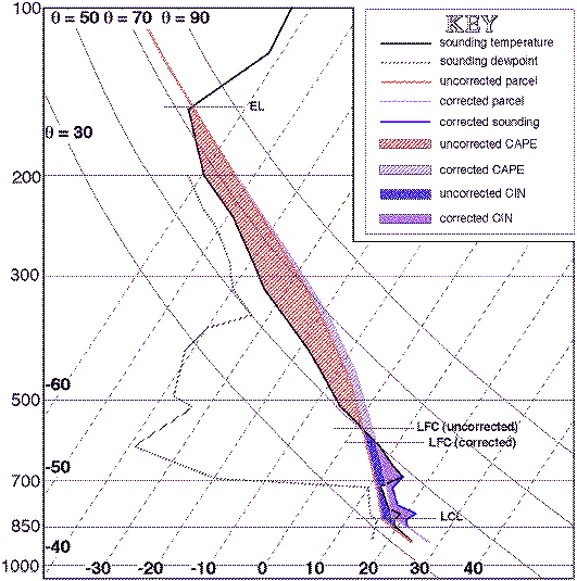
Figure 1. Schematic sounding, showing the processes with and without the virtual correction (see the key). The parcel ascent curve is for the surface parcel.
There are several things to note about this schematic ... the mixing ratio generally decreases as one gets up into the mid- and upper troposphere, and the schematic example sounding shown is quite dry above the moist surface boundary layer, so the virtual correction to the sounding curve pretty much becomes negligible above the moist layer. However, for the parcel ascent curve above the saturation point (LCL), the parcel is assumed to be saturated, so there is a non-negligible virtual correction through a much greater depth than there is for the sounding. The EL for the corrected ascent curve is virtually the same as for the uncorrected curve because the EL generally is in the upper troposphere, where the mixing ratio even in a saturated situation is negligible. However, for this example, the LFC is notably lower whereas the LCL remains the same, for reasons already discussed. The result is that the corrected CAPE is notably higher, whereas the corrected CIN is not all that much different. Not all soundings will have precisely these characteristics, as discussed in Doswell and Rasmussen (1994) but many will in situations where deep convection is possible.
Also, observe that the apparent saturation point of the corrected parcel ascent curve is shifted to the right on the Skew-T, Log p diagram as a result of the virtual correction. Because movement to the right on the diagram is toward higher mixing ratios, this might suggest to the unwary that the implied mixing ratio associated with the saturation point has increased. This appearance is somewhat deceptive; the true saturation point remains unchanged, but if we want to compute the density at the saturation point, we must use the virtual temperature, not the actual temperature. All we are doing is applying the virtual correction to the parcel ascent temperature curve. Since the correction is always non-negative, this results in a rightward shift of the trace (each point moves to the right at the same pressure where it started), but this does not imply an increase in the actual dewpoint. The virtual correction is never applied to the sounding dewpoint trace! Keep in mind that the virtual correction is only used to calculate density, not to infer the thermodynamics of the saturation point during the psuedo-real parcel ascent.
The process of making the virtual correction to the parcel ascent trace occurs only after having computed the uncorrected parcel ascent curve. Never use the corrected sounding profile to compute the parcel ascent curve! The virtual correction to the parcel ascent curve uses the dewpoint of the ascending parcel (which is along the mixing ratio line below the saturation point, and is equal to the temperature along the moist adiabat which the parcel ascends at and above the saturation point). The LCL is the same as that found using the uncorrected parcel ascent process, whereas the CAPE, CIN, LFC, and EL should be found from the corrected sounding and parcel ascent traces.
Note added: 21 April 2008
Another issue concerns the effect of making the virtual correction on variables like CAPE and CIN. As noted in the 1994 paper with Erik Rasmussen, the use of the virtual correction doesn't necessarily always have a significant effect on such calculations, but in some situations it might make a difference that could influence a forecaster's decision-making. Consider the following example (supplied to me by Rich Thompson - Thanks, Rich!) of a sounding:
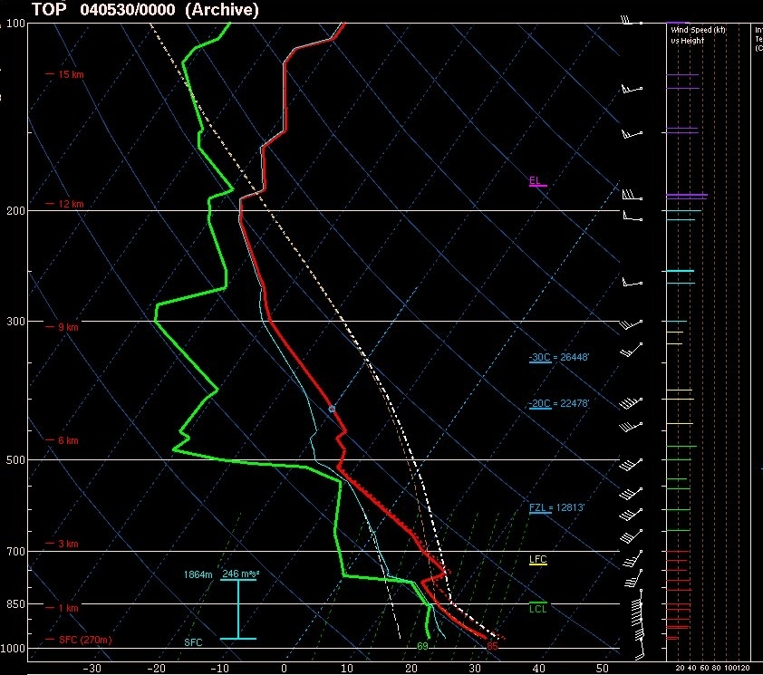
Figure 2. Observed sounding at 00Z from Topeka, KS on 30 May 2004, illustrating the effect of the virtual correction on the calculated CIN for a mixed layer parcel.
The format of the plotting routine shows the uncorrected parcel ascent curve (in a dark yellow) and the corrected parcel ascent curve (in white) for a mixed layer parcel. A potentially interesting issue is the observation that the uncorrected parcel has some modest but not negligible amount of CIN, whereas the corrected parcel CIN has only a very tiny amount. The surface parcel has 0 CIN, in part because of the relatively deep superadiabatic contact layer. On this particular day, tornadic supercells developed in northern Kansas.
The idea that a nearly "uncapped" sounding implies that deep convection is probably already underway or may be imminent is based on the very simple notions of basic parcel theory. In my experience, small CIN does not inevitably associate with the development of deep convection. Consider the following example from OUN on the evening of 26 April 1991. Major tornadic storms were ongoing in the northern 1/3 of Oklahoma on into southern Kansas during this rawinsonde ascent, and also developed just on the Texas side of the Red River. In between, however, near Norman, no sustained deep convection ever developed, even though the OUN sounding is very nearly uncapped. The reasons for this are not obvious, but it certainly illustrates that calculated CIN is not definitive evidence for or against the likely initiation of deep convection.
Norman, OK (OUN) sounding from the evening of 26 April 1991. Compare the CIN values using the corrected (CINV) and uncorrected (CINS) ascent curves - small values indicate nearly uncapped conditions. Depending on the details of precisely how the calculations are done, I'd say that this sounding is essentially uncapped. Also note the difference between the corrected CAPE (CAPV) and the uncorrected value.
Every situation is different, and we often don't have enough information on hand to know the reasons for this departure from the apparent "predictions" derived from parcel theory-based diagnostic parameters. But in my experience, it's not at all uncommon.
I should point out that both corrected and uncorrected CIN come from the same data: the sounding. They are slightly different ways to compute these variables -- one corrects for the effect of water vapor on density while the other does not. In principle, if buoyancy is at issue, accounting for the effect of water vapor is "more correct" than ignoring it. Should the interpretation of CIN be the same for the two different methods for calculating variables? I think not. It's not a matter of which is "more correct" for the particular application -- neither is correct, since parcel theory is such a bad model of real convection. That simple theory ignores a lot of things, as discussed by Rasmussen and Doswell (1994) as well as Doswell and Markowski (2004). The use of parcel theory-based diagnostics in a literal, quantitative sense to assess the likelihood for deep, moist convection is potentially perilous, especially if all one considers is indices and parameters computed from the sounding - see the paper:
Doswell, C.A. III, and D.M. Schultz, 2006: On the use of indices and parameters in forecasting severe storms. Electronic J. Severe Storms Meteor., 1(3), 1-22.
which is available at the same location as my other publications cited here.
Note added: 15 May 2008
Please keep in mind some (hopefully) simple notions.
H
___________________________
* I'm describing the calculation of CAPE as the determination of relative buoyancy. That is, CAPE involves the difference in temperature between the parcel and some base state sounding (in this case, the "environmental" sounding). There is no simple way to define the notion of an "environment" for convective situations and, therefore, the notion of the base state sounding is actually rather nebulous and is actually unphysical. An ascending parcel does not need to know its temperature relative to anything outside of the vertical column within which it is found, in order to be buoyant. In reality, buoyancy is an unbalanced vertical pressure gradient force, and so an ascending parcel's buoyancy must be independent of any "environment" or "base state"! The traditional derivation of buoyancy as the difference in temperature between the parcel and the "environment" is an incomplete and misleading representation of buoyancy. Paul Markowski and I have published a paper on this subject.